I mentioned the process automation concept of ISight in a previous simulation automation blog. ISight is an open source code simulation automation and parametric optimization tool to create workflows that automate the repetitive process of model update and job submission with certain objectives associated with it. The objective could be achievement of an optimal design through any of the available techniques in ISight: Design of experiments, optimization, Monte Carlo simulation or Six Sigma. In this blog post, I will be discussing various value added algorithms in DOE technique; I will discuss other techniques in future blogs.

Why design of experiments

Real life engineering models are associated with multiple design variables and with multiple responses. There are two ways to evaluate the effect of change in design variable on response: Vary one at a time (VOAT) approach or Design of experiments (DOE) approach. The VOAT approach is not viable because:

• This approach ignores interactions among design variables, averaged and non-linear effects.
• In models associated with large FE entities, each iteration is very expensive. VOAT does not offer the option of creating high fidelity models with a manageable number of iterations.

With the DOE approach, user can study the design space efficiently, can manage multi dimension design space and can select design points intelligently vs. manual guessing. The objective of any DOE technique is to generate an experimental matrix using formal proven methods. The matrix explores design space and each technique creates a design matrix differently. There are multiple techniques which will be discussed shortly and they are classified into two broad configurations:

• Configuration 1: User defines the number of levels and their values for each design variable. The chosen technique and number of variables determines number of experiments.
• Configuration 2: User defines the number of experiments and design variables range.

Box-Behnken Technique

This is a three level factorial design consisting of orthogonal blocks that excludes extreme points. Box-Behnken designs are typically used to estimate the coefficients of a second-degree polynomial. The designs either meet, or approximately meet, the criterion of rotatability. Since Box-Behnken designs do not include any extreme (corner) point, these designs are particularly useful in cases where the corner points are either numerically unstable or infeasible. Box-Behnken designs are available only for three to twenty-one factors.

Central Composite Design Technique

 The Central Composite Design technique is a statistically based technique in which a 2-level full-factorial experiment is augmented with additional points. In the Central Composite design technique, a 2-level full-factorial experiment is augmented with a center point and two additional points for each factor (called “star points”). Therefore, five levels are defined for each factor, and to study n factors using Central Composite Design requires 2n + 2n + 1 design point evaluations. Although Central Composite Design requires a significant number of design point evaluations, it is a popular technique for compiling data for response surface modeling because of the expanse of design space covered and the higher-order information obtained.

The center and star points are added to acquire knowledge from regions of the design space inside and outside the 2-level full-factorial points, allowing for an estimation of higher-order effects (curvature). The star points (S) are determined by defining a parameter “a” that relates these points to the full-factorial points by:

S upper = b + (u – b) × a

S lower = b – (b – l) × a

b = baseline design

l = lower factorial point

u = upper factorial point

l < b < u

Latin Hypercube Technique

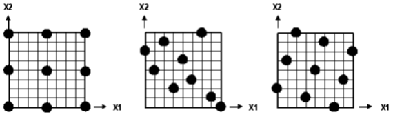
The Latin Hypercube technique is a class of experimental designs that efficiently samples large design spaces. In the Latin Hypercube technique, the design space for each factor is divided uniformly (the same number of divisions, n, for all factors). These levels are randomly combined to specify n points defining the design matrix (each level of a factor is studied only once). For example, the following figure illustrates a possible Latin Hypercube configuration for two factors (X1, X2) in which five points are studied. The Latin Hypercube technique allows the designer total freedom in selecting the number of designs to run.

Optimal Latin Hypercube Technique

The Optimal Latin Hypercube technique is a modified Latin Hypercube where the combination of factor levels for each factor is optimized, rather than randomly combined.

In the Optimal Latin Hypercube technique, the design space for each factor is divided uniformly (the same number of divisions, n, for all factors). These levels are randomly combined to generate a random Latin Hypercube as the initial DOE design matrix with n points (each level of a factor studies only once). An optimization process is applied to the initial random Latin Hypercube design matrix. By swapping the order of two factor levels in a column of the matrix, a new matrix is generated and the new overall spacing of points is evaluated. The goal of this optimization process is to design a matrix where the points are spread as evenly as possible within the design space defined by the lower and upper level of each factor.

This type of matrix is not reproducible (unless the same random seed is reused) because the Optimal Latin Hypercube begins as a random Latin Hypercube and is optimized using a stochastic optimization process.

 Data File Technique

This method allows users to incorporate their own set of design points into ISight by using an external file. The file could be any text file having data in rows depicting number of data points and data in columns depicting design variable values for each data point.